Before starting to write a blog post I always ask myself - “What is the added value?”. There is a lot of awesome ML material out there. And a lot of duplicates as well. Especially when it comes to all the flavors of Deep Reinforcement Learning. So you might wonder what is the added value of this two part blog post on Deep Q-Learning? It is threefold.

1. We will review all the ingredients of modern value-based Reinforcement Learning (RL). Starting with Tabular Q-Learning (Watkins & Dayan, 1992) we will travel through the world of value function approximator and finally end up with all the ingredients to the state-of-the-art Rainbow (Hessel et al., 2018) algorithm in a single blog post ().

2. In a future post we will further gain insights into the effect of the hyperparameter choices in Deep Q-Learning. In order to do so, we will deal with the simplified gridworld shown below. You can find the corresponding code in this repository ().

   

3. After having become experts in ablation studies and fiddling around with hyperparameters, we will have a closer look at 3 recent papers shining some more empirical as well as theoretical light on the divergence behavior in Deep Q-Learning dynamics ().

Let’s get rolling… or updating ! But before one note of caution: We cover quite a lot of ground, so feel free to jump around and skip sections which you feel like you have already mastered.

• Setting the Stage: The Reinforcement Learning Problem
  • The World as a Markov Decision Process
  • Problem Formulation & Dynamic Programming
• (Deep) Q-Learning: A Historical Overview
  • Tabular Q-Learning
  • Fitted Q-Learning
  • Deep Q Networks (DQN)
  • Double DQN (DDQN)
  • Prioritized DQN (PER)
  • Dueling DQN
  • Noisy Nets
  • Categorical DQN
  • Rainbow
• The One Equation Summary aka TL;DR
• References

Setting the Stage: The Reinforcement Learning Problem

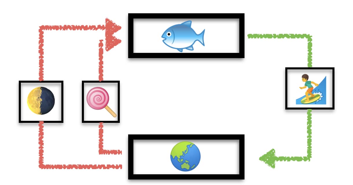Our () everyday lives are full of perceptual experiences of our surroundings (). We constantly make decisions () that change how & what we experience (). Crucially, we get rewarded () for good choices and sometime punished for bad ones. Feedback is in many ways crucial to our existence. This feedback can be extrinsic (e.g. monetary or the satisfaction physical needs) or intrinsic (e.g. motivation, curiosity or social aspects). We adapt our behavior to such cues. Why? To fulfill our hedonistic desires () or simply to survive (). And Reinforcement Learning describes a computational framework for exactly these reward-based adaptation dynamics.

The World as a Markov Decision Process

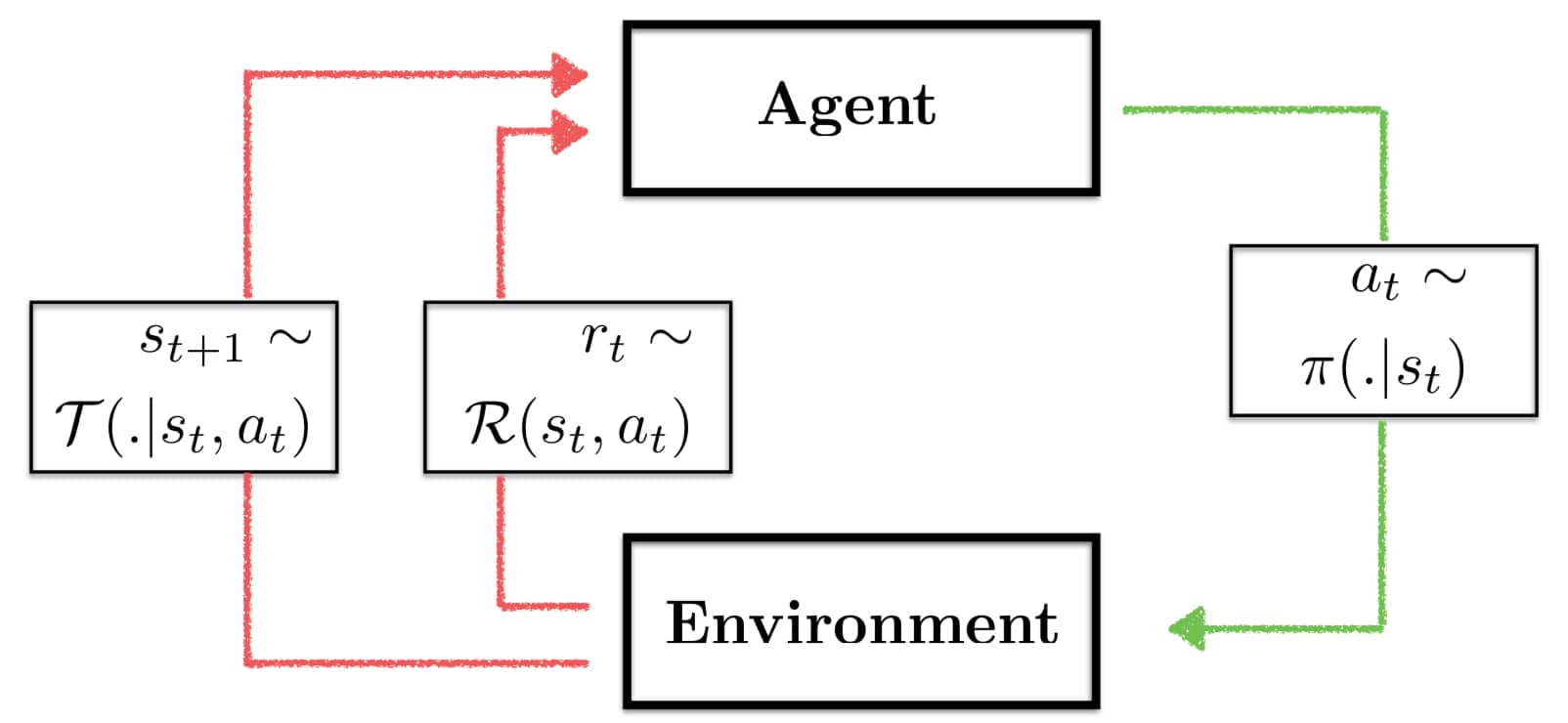
Most traditional RL approaches are situated within the more general framework of Markov Decision Processes (MDP). An MDP consist of the tuple $(\mathcal{S}, \mathcal{A}, \mathcal{T}, \mathcal{R}, \gamma, p_0)$ where:

• $\mathcal{S}$: Denotes the state space in which an agent is situated at a current point in time $t$, i.e. $s_t \in \mathcal{S}$ and informally , $\in \mathcal{S}$.
• $\mathcal{A}$: Denotes the action space from which an agent is allowed to choose its next move from, i.e. $a_t \in \mathcal{A}$ and informally $\in \mathcal{A}$.
• $\mathcal{T}$: Denotes the transition kernel which provides you with the probably of transitioning to a state $s’$ given that the agent is currently in state $s$ and takes action $a$, i.e. $p(s’ \mid s, a)$ describes informally the probability of $\to$ given .
• $\mathcal{R}$: Denotes the reward function which given a state transition $s, a, s’$ issues a reward to the agent (). This reward can be stochastic or deterministic.
• $\gamma$: Denotes a factor $\gamma \in [0,1)$ with which rewards accumulated in future timesteps is discounted. From an economics point of view returns we can obtain today are associated with less uncertainty and can directly be consumed. More fundamentally the discount factor can viewed as a survival probability which incorporates some fundamental time uncertainty of the agent.
• $p_0$: Denotes the initial state distribution for $t=0$, i.e. where the agent is initialized.

Given a state the agent chooses the next action according to a policy $\pi(a \mid s)$. It can be deterministic, which means that given a state the agent will always choose a specific action. Or it can be stochastic, where the next action is sampled from the distribution.

So what exactly is Markovian about this MDP and does this restrict us in modeling reward-based learning? The next state transition is assumed to only depend on the state and action of the current time step. So what if the agent had to pickup a key twenty steps ago to open a door right now? As long as the key is part of the current state that is not a problem. If not we are in danger. Velocity in ATARI games is another of such examples. A single frame cannot tell you in which direction and how fast a ball is moving. Mhmm… that is a bummer. But wait! We can infer velocity from two frames! So as long as a state is represented cleverly all dynamics can be described as Markovian. Finding the right composition of states can be challenging though.

Problem Formulation & Dynamic Programming

So how can we articulate all of our hedonistic desires? We need some maths here! Two key quantities of interest in RL are the state value function $V^\pi(s)$ and the action value function $Q^\pi(s,a)$:

where $V^\pi(s) = \sum_{a \in \mathcal{A}} \pi(s,a) Q^\pi(s,a)$ . Intuitively, $Q^\pi(s,a)$ denotes the reward that one is expected to obtain when starting from state $s$ you first take action $a$ and only afterwards continues to follow the current deterministic policy $\pi$. $V^\pi(s)$, on the other hand, directly selects actions according to the policy. Ultimately, in order to solve the Reinforcement Learning problem we are interested in the optimal behavior policy $\pi^\star$ that is derived by maximizing this expression:

This optimization problem is termed the Reinforcement Learning problem. Given this setup, classical Dynamic Programming (DP) algorithms alternate between evaluating a given policy (the prediction problem) and performing a greedy improvement upon the current policy. This procedure is known as generalized value iteration and is guaranteed to converge. (Note: This is due to the fact that one can show that the Bellman operator in the above equation is a $\gamma$-contraction and assured to converge to the fixed point in $Q^\star$). The downside of DP methods is that they require access to the transition dynamics of the environment $\mathcal{T}. And these are usually not given. So what is the solution? It is sample-based learning!

(Deep) Q-Learning: A Historical Overview

Everyone who begins to dabble into Deep RL first encounters basic Q-Learning. Q-Learning is a value-based RL method. Instead of directly optimizing the behavior of an agent (as is done policy in policy-based methods), one does so indirectly by refining the action value estimates $Q(s,a)$. The beauty of this lies in the observation that if we have the optimal value estimates, we can simply act greedy with respect to the action choice!

So learning a better estimate of the expected state-action pair values allows us to end up with better policies. We are now going to stepwise extend our intuition as well as algorithmic knowledge about different Q-Learning ideas.

Tabular Q-Learning

Tabular Q-Learning represents the action value function $Q(s,a)$ as a lookup table and updates the individual entries with the help of simple temporal difference (TD) error learning:

The expression $Y_k = r + \gamma \max_{a’ \in \mathcal{A}}Q(s’,a’)_k$ is usually referred to as the one-step target and the difference between the target and our current estimate, $\delta_k(s,a,r,s’) = Y_k - Q(s,a)_k$ is the TD error. $\eta \in (0, 1]$ denotes the learning rate, i.e. how much we scale the prediction error before updating our estimate. This process is often called “bootstrapping”. It refers to us updating our $Q(s,a)$ estimate with another estimate, namely $Q(s’,a’)$. Thereby, we “bootstrap” from our own current state of knowledge. (Note: This is not to be confused with the bootstrapping terminology from computational statistics which calculates a statistic based on Monte Carlo samples from the overall data. Random Forests for example use bootstrapping aka bagging to estimate different trees based on subsampled datapoints as well as dimensions.) In early work Watkins & Dayan (1992) showed that these simple one-step updates are guaranteed to converge to $Q^\star$ … under some conditions:

1. Every state-action pair is visited often enough (infinite times in the limit).
2. The learning rate $\eta$ follows a schedule that satisfies the Robbins-Monroe criteria.

We have already learned about the differences between value-based and policy-based methods. Another important distinction is the one between on- & off-policy methods as well as exploration. Convergence criterion 1 requires the agent to visit many different states with the help of many different actions. But ultimately, the optimal policy $\pi^\star$ might not want to do so .

Therefore, in off-policy learning we introduce a second policy that is used to collect the transitions needed to update the policy. This policy $\beta$ is called the behavior policy since it is the policy that determines the behavior of the agent during training. So we collect data $<s,a,r,s’>$ with $\beta$ and update $\pi$ afterwards. One well-known way of doing so is having $\beta$ be $\epsilon$-greedy. At each time step on samples an $\vartheta \sim \mathcal{U}[0,1]$.

If $\vartheta$ is greater than $\epsilon$ than the agent executes an action following $\pi$. Otherwise, they randomly choose an action from $\mathcal{A}$. We can directly see that in this case the behavior policy is also responsible for trading off exploration & exploitation. Starting from a large $\epsilon \approx 1$ one usually anneals it down to a small value $\approx 0.05$ over the course of the learning. Intuitively. in the beginning of learning one wants to sample from all over the state and action space. Later on as we progress, it makes more sense to zoom into the already good behavior and stay more “on-policy”.

In some really outstanding work Schultz et al. (1997) showed that the activity of dopaminergic neurons correlated with this reward prediction error $\delta$. In their experiments mice performed a reward-based task. And whenever the expectation of a reward (as measured by $V(s)$) and the actual issued reward (as measured by sweet liquid drops) were not aligned the dopamine neurons fired proportionally. This observation is termed the Dopamine Reward Prediction Error Hypothesis & has been the entry point for many ideas from computational psychiatry to study trial-based learning within the formal framework of RL. The discount factor and learning rate can be viewed as subject-specific parameters which are optimized to fit the actual behavior within an experiment. Dramatic “parametric” deviations can then be viewed as an indicator for mental disorders. Pretty cool right? Back to theory now.

Tabular Q-Learning only updates a single value per transition $<s, a, r, s’>$. As the dimensionality of the state space $\mathcal{S}$ grows, this becomes very sample inefficient. So what can we do? We need to generalize across the state space! By assuming smoothness of the action value estimates across states and actions, we can approximate the value function with a set of parameters $\theta$:

These parameters might characterize a set of coefficients corresponding to a polynomial or the weights of different network layers. The general idea can be summarized as follows: In order to obtain good value estimates across the state space, we need to generalize from the experienced transitions. Function approximators have proved themselves to be very capable of doing something similar within supervised learning. So let’s try them out!

Fitted Q-Learning

The next question becomes how do to learn the parameters describing our approximate value function? In seminal work Gordon (1996) formulated the Mean Squared Bellman/TD error objective as:

with $Y_k = r + \gamma \max_{a’ \in \mathcal{A}} Q(s’, a’; \theta_k)$. The parameters are then updated using simple SGD:

This update can be rather simple when using a form of polynomial approximation or more complex involving backpropagation (aka the memory efficient application of the chain rule). So one might ask why didn’t Deep Q-Learning already take off in the 20th century? The two main reasons were the following:

1. Sample inefficiency: Performing single batch or even online updates and then discarding the transitions is extremely inefficient and will lead to learning instabilities due gradients with large variance. Second of all it will lead to overfitting of the most recent transitions and a form of catastrophic forgetting.
2. Moving Target Dilemma: In order to compute the target we need the most recent estimate of the Q function $Q(s,a;\theta_k)$. And since $\theta$ changes after every update, the target changes as well. This might not necessarily be a problem considering small learning rates, but since deep nets are so flexible it can come to overgeneralization which can lead to strong instabilities.

Interestingly, in the tabular case all entries in the lookup table can be interpreted as the set of parameters $\theta$. In this case $\nabla_{\theta_k} Q(s,a;\theta_k)=1$ and the gradient based update boils down to the simple tabular Q-Learning update.

Takeaway: What really stuck with when I first started reading about DQNs was the fact that most of the underlying theory was already out there in the mid-90s. Old concepts come back! Many of recent ideas in Deep RL simply revive existing ideas from the beginning of the century.

Takeaway: In order to tame the beast of high-dimensional state spaces, flexible and generalizing value function approximators were introduced. These, on the other hand, bring their own kind of beastly problems with themselves which can render the learning dynamics inefficient as well as unstable.

Deep Q Networks (DQN)

So what had to happen for Deep Reinforcement Learning to rise? Mainly two major innovations by Mnih et al. (2013) were necessary:

1. Experience Replay (ER): Li et al. (1992) introduced a buffer system that acts as a form of dataset which is composed of transitions sampled from in an off-policy fashion (e.g. $\epsilon$-greedy action selection using the current) policy. ER is loosely inspired by hippocampal replay observed in place cells of sleeping mice (really exciting stuff!). Instead of “tossing away” all transitions after using them in a single update, they are stored and later “replayed”. More specifically, we keep a dataset $\mathcal{D} = {<s, a, r, s’>}$ and add new transitions to it as the agent moves around:

   The buffer has capacity $N^{replay} \in \mathbb{N}$. As we fill the buffer up, it will boil over and the oldest transitions will be forgotten. Learning then involves uniformly sampling a mini-batch of transitions from the buffer $s, a, r, s’ \sim \mathcal{U}(\mathcal{D})$ and computing $\nabla Q(s,a; \theta_k)$. The samples come from a mixture of non-stationary off-policy distributions and thereby it is quite surprising, that this still allows for efficient learning.

2. Target networks: Instead of using the most recent estimate of the Q function one can also save an older version of the network and use that older version to compute the targets. After a certain fixed number of iterations that “target” network’s parameters are then set to the most recent value network’s parameters.

   \[Y_k^{DQN} = r + \gamma \max_{a' \in \mathcal{A}} Q(s', a'; \theta_k^-)\]

   The parameters $\theta_k^-$ are set to the updated online parameter $\theta_k$ every $C \in \mathbb{N}$ iterations. Alternative is provided by Polyak averaging: $\theta^-k = \tau \theta_k + (1-\tau) \theta{k-1}^-$! Empirically, it has been shown that this slowly changing network allows to stabilize the learning dynamics. Intuitively, function approximation wonderfully allows to generalize across the state space. Unfortunately, it can also happen to lead to “overgeneralization”.

These two innovations combined with a bunch of hacks (frame skipping, reward clipping as well as gray scaling of frames) ultimately led to the breakthrough of DQNs. It achieved super-human performance on many of the 57 ATARI benchmark games, provided a substantial ingredient to later iterations of AlphaGo and also serves as a foundation for continuous control Actor-Critic algorithms such as DDPG. All what follows are extensions and improvements of this base module.

Double DQN (DDQN)

It is true that there are not that many strong theoretical results when it comes to RL using non-linear value function approximators. But there are quite a few that hold for the simpler tabular or linear approximator case. And their intuition often times holds or even gets amplified when using non-linearities. In seminal work van Hasselt et al. (2010) generalized a previous result by Thrun & Schwartz (1993), proving an innate overestimation bias in Q-Learning resulting from noise within the environment as well as estimation error induced by approximating the true value function.

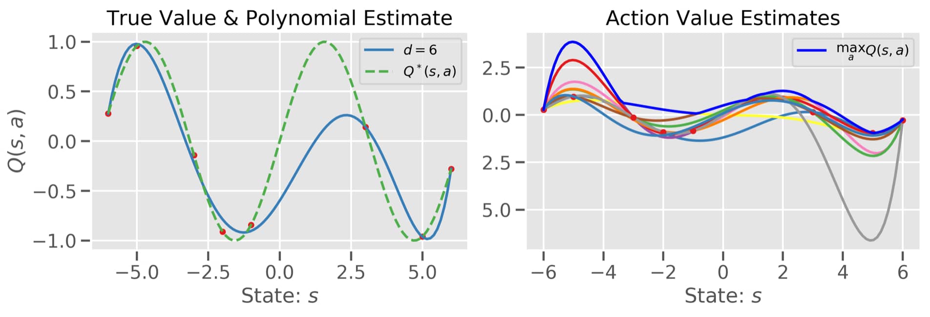
Imagine the following scenario (see above figure): We (as the designers of this thought experiment) have access to the true optimal action value function $Q^\star$ (green line on the left-hand side). And we know that for a set of 10 actions it takes the same value for a specific state. And then let’s say that the agent has access to the exact values (!) for 6 different states for each action (so 60 state-action pairs). For each action, the agent then fits a polynomial of degree 6 to come up with his action value estimates (see the rainbow of different curves on the right-hand side figure). If we then take the max over the action space, we end up with the dark blue line.

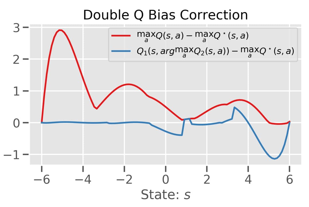Intuitively, when bootstrapping we would like to make use of $\max_a Q^\star(s,a)$ to update our current value estimate. But we only have access to $\max_a Q(s,a)$. So the smaller the difference $\max_a Q^\star(s,a) - \max_a Q(s,a)$ the better! And now have a look at this ugly plot! The difference for most states is positive! Damn it - the overestimation is obvious. Van Hasselt et al. (2010) and later Van Hasselt et al. (2016) showed that the key to this bias lies in the usage of the max operator when computing the bootstrap target:

By rewriting the DQN target formulation we can directly observe that we are using the target network twice: Once to greedily select the next action taken and once to evaluate the bootstrap estimate. So where does the overestimation kick in? The max operation will greedily prefer actions which have a high value estimate. But that estimate is noisy. Hence, it can happen that this action does not correspond to the true value function and since we are also evaluating the value of taking that action with the noisy estimate, the noise will be amplified and manifests itself in the learning dynamics. A simple ad-hoc fix to this problem of bootstrapping is to disentangle evaluation and action selection. In practice, this means that one network (say $\theta_1$) is used to perform the argmax and another network (say $\theta_2$) will be used to evaluate that selected action. If we do so we can mitigate the overestimation bias (see the blue line in the above figure). So do we have to keep another network around? The answer is yes and no. We already have a target network which we can use for that!

Takeaway: The speed with which we update the target network crucially affects the quality of the disentanglement between selection and evaluation of an action.

Prioritized DQN (PER)

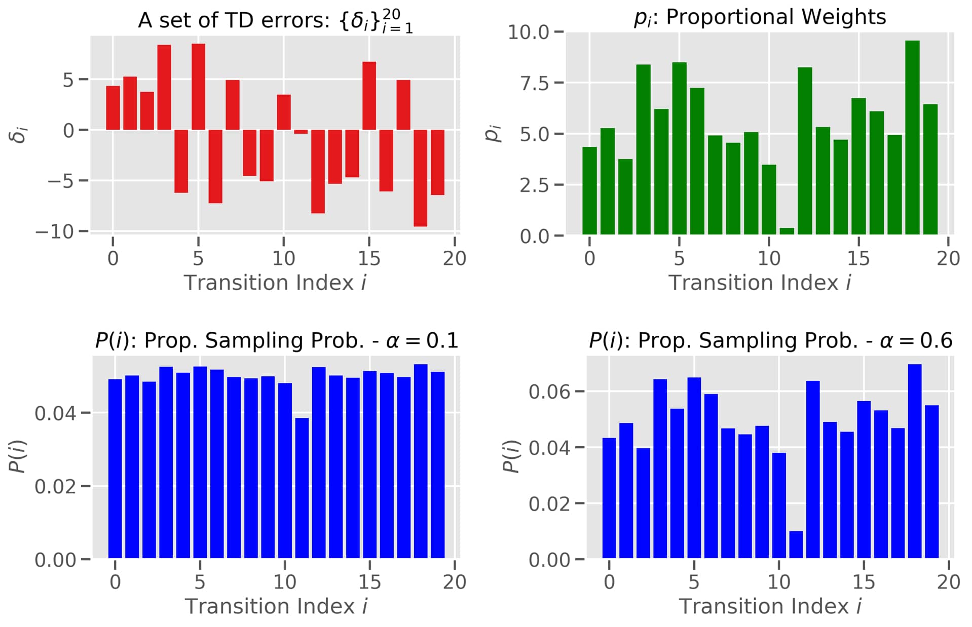
Memory in Deep Q-Learning is composed into two parts: storage and computation. Transitions are stored in a sliding window fashion. And computation is done using a uniform sampling distribution. Uniform sampling from the ER buffer is the most simple form of calculating an off-policy Monte Carlo estimate one can come up with. Schaul et al. (2015) try to improve this. Instead, they propose sampling transitions proportionately to a measure of associated “learning progress”. A potential measure is the magnitude of the TD error ($\mid \delta(i) \mid$) associated with a transition $i$! The new sampling distribution $P(i) = \frac{p_i^\alpha}{\sum_k p_k^\alpha}$ can then be obtained in two different ways

• Rank based: $p_i = \frac{1}{rank(i)}$ with the rank being obtained from the sorted $\mid \delta_i \mid$
• Proportionately: $p_i = \mid \delta(i) \mid + \epsilon$ where $\epsilon$ ensures that each transition has a non-zero probability of being sampled.

Intuitively, the temperature parameter $\alpha$ in this Boltzmann distribution controls the amount of “prioritization”, i.e. how much we prefer large magnitude TD transitions over smaller ones:

• $\alpha \to 0$: No prioritization leading to uniform sampling as in ER.
• $\alpha \to 1$: Full prioritization leading to transitions with large magnitude TD error being sampled more frequent.

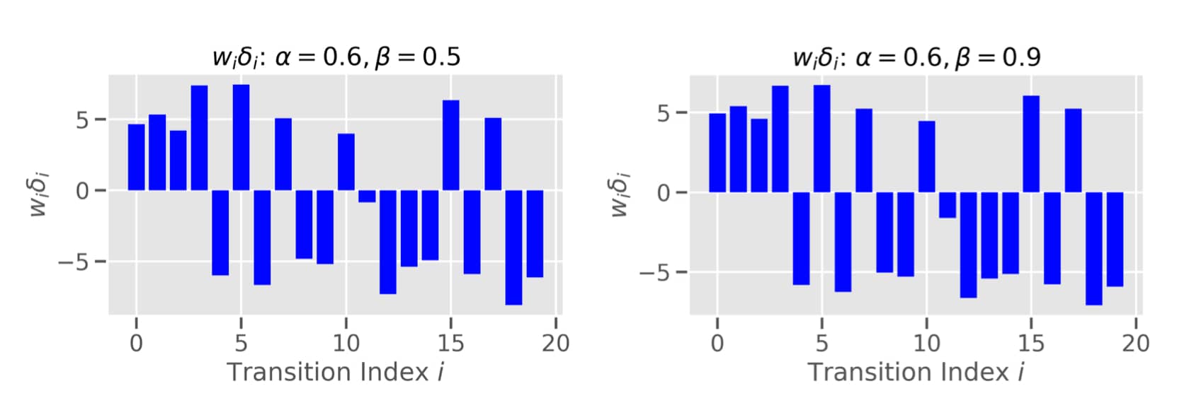
Importantly, when prioritizing we are no longer sampling transitions according to the mixture of off-policy distributions that filled our buffer $\mathcal{U}(\mathcal{D})$. Schaul et al. (2015) state that this introduces bias (while reducing gradient variance!). Intuitively, the more we prioritize the stronger the degree of “off-policiness”. They propose a simple importance sampling correction which rescales the TD errors:

where $w_i = (\frac{1}{N} \frac{1}{P(i)})^\beta$ and for stability purposes we standardize such that $ \tilde{w}_i = \frac{w_i}{max_i w_i}$. $\beta$ mitigates the impact of the prioritization and is usually linearly to 1 (usually starting at 0.4). Checkout the influence on the weighted TD errors below:

A way I like to think about the effect of $\beta$ and the annealing schedule is in terms of yet another bias-variance trade-off in RL. Setting $\beta=1$ reduces the whole procedure back to uniform ER. $\beta$ smaller but close to 1, on the other hand, “lets through” a little bit of IS introduced bias while reducing the variance. And the annealing schedule gradually reduces the bias. One reason why this might be effective is the interplay with the capacity of the replay buffer. In some small-scale experiments I found that PER really helps to focus the SGD updates in the initial learning where there are many “useless” transitions in the buffer (such as bumping into walls). Later on, as the “quality” of the buffer increases the effect diminishes - and it makes sense to be closer to uniform sampling, i.e. $\beta=1$.

The authors mention that there might be more fruitful ideas out there revolving around the storage aspect of ER. The somewhat ad-hoc moving window which kicks out transitions in their respective order could potentially be improved by accounting for state-transition entropy within the buffer system.

Takeaway: Prioritization and thereby the degree of off-policy can be controlled by $\alpha$ and $\beta$. Setting $\alpha=0$ or $\beta=1$ reduces the extend of off-policy we are when updating the value estimates. This will be a reoccurring story in the next blog post where we discuss the Deadly Triad of DRL.

Dueling DQN

All improvements up to now focused on improving the learning algorithm used in Deep Q-Learning. Wang et al. (2015), on the other hand, attempt to improve by asking whether there are Deep Learning architectures that are more suited than others. But before we continue, we first need to introduce the notion of the advantage of a state-action pair $A(s,a)$:

The advantage of an action measures the relative importance of each action given state $s$. Since $V^\pi(s) = \sum_{a \in \mathcal{A}} \pi(s,a) Q^\pi(s,a)$ we have that $\mathbb{E}_{a \sim \pi} [A^\pi(s,a)] = 0$.

Wang et al. (2015) motivate their approach by the simple observation that many state transitions in ATARI games are action independent. Hence, often times $A^\pi(s,a) = 0$. When propagating gradients through the network architecture we might therefore run into trouble. The authors therefore propose to split the network architecture into two streams: Value and advantage stream. This allows us to better learn state value estimates regardless of the action taken. One way I like to think about the two streams is similar to how Resnet architectures work. Given the state value estimate, obtaining the action value estimate is a form of residual effort mediated by the advantage of an action. Splitting the streams then provides “architectural support” to propagate gradients without having to disentangle the impact of the chosen action.

So how is this actually done? Observe that the equation $Q^\pi(s,a) = A^\pi(s,a) + V^\pi(s)$ is not identifiable. That means we cannot uniquely recover either $A^\pi(s,a)$ or $V^\pi(s)$. In order to mitigate this problem, one can make use of the fact that the advantage has to be 0 for the chosen action. This follows from \(a^\star = arg\max_a Q(s,a) = arg\max_a A(s,a)\) and therefore $Q(s,a^\star) = V(s)$.

Wang et al. (2015) note that learning dynamics can be stabilized by further replacing the max operator by the mean over the action space. Furthermore, the subtraction of the constant does not change the relative ordering of the values and therefore, greedification still arrives at the same action selection.

Takeaway: In my mind this piece of work highlights the many different angles from which one can approach the RL problem. Architectures, optimization, exploration, learning rules, etc. are all different faces of the same problem.

Noisy Nets

So what about exploration? Up to know all approaches used the linear schedule of $\epsilon$-greedy exploration described above. Fortunato et al. (2017) showed that there is something smarter to do. More specifically, they alter all the fully-connected linear layers in the network to include an additional set of parameters $\tilde{W}, \tilde{b}$ which are elementwise multiplied with sampled Gaussian noise:

Intuitively, the set of additional parameters filter how much noise is allowed to affect the action choice of the agent. And they are learned end-to-end with backpropagation. Hence, the network can learn at which stages of learning to explore more and at which to explore less.

Takeaway: Learning when to explore is super cool. Learning where to explore would be even cooler!

Categorical DQN

When I first got to read Bellemare et al. (2017) it struck me like thunder - Why do we actually always optimize the expectation of the summed discounted returns when there is a full distribution to work with? Instead of reducing the random return $Z$ to its mean $Q$, distributional approaches intend to model the full distribution (or a discrete approximation with $N$ atoms ($z_i, p_i$):

The main benefits of this approach is in capturing multiple modes in the value distribution and stabilizing the noise introduced by value function approximation. The parametrization of the probabilities $p_i$ associated with each atom’s location $x$ is then optimized to match the Bellman projected probabilities after bootstrapping, $m$ (please excuse the lack of detail here):

In their work Bellemare et al. (2017) derive a contraction proof for the Distributional Bellman Operator in the max form of the Wasserstein (or Earthmover) distance. Since Wasserstein distance cannot easily be optimized by SGD, their implementation makes use of the easy to compute KL divergence instead. Thereby, throwing much of their hard theoretical work over board. In more recent work this limitation is overcome by no longer optimizing the probability $p_i$ assigned to specific atoms but by changing the location of the atoms/quantiles (Dabney et al., 2017a, 2017b).

Takeaway: There are many exciting under-explored paths in DRL which can account for different levels of risk sensitivity. This might allow for alternative ways exploration via risk seeking behavior and survival behavior via risk averse behavior.

For everyone who wants to learn more about distributional RL I recommend reading this great blog post by Massimiliano Tomassoli. It gives a lot more detailed and intuitive explanations than I can fit in here.

Rainbow

Rainbow (Hessel et al., 2018) was a recent paper which improved upon the state-of-the-art (SOTA) by combining all the approaches outlined above as well as multi-step returns. Multi-step returns allow to trade off the amount of bootstrapping that we perform in Q-Learning. More, specifically $k$-step update for simple tabular Q-Learning can be written as:

The larger $k$, the less we bootstrap. Many of the stepwise improvements are somewhat orthogonal to each other and can be combined! Most combinations appear to be fairly hyperparameter insensitve. Furthermore, they find that Prioritized ER and multi-step returns provide the most crucial performance boost.

The One Equation Summary aka TL;DR

In this blog post we took a deep dive into Deep Q-Learning. Below you find a figure summarizing the key elements of each algorithm:

See you next time for the second half of this series, in which we cover some hyperparameter experiments and discuss some theoretical foundations of the divergence behavior observed in Deep Q-Learning!

References

1. Dabney, W., M. Rowland, M. G. Bellemare, and R. Munos. (2018): “Distributional Reinforcement Learning with Quantile Regression,” Thirty-Second AAAI Conference on Artificial Intelligence, .
2. Dabney, W., G. Ostrovski, D. Silver, and R. Munos. (2018): “Implicit quantile networks for distributional reinforcement learning,” arXiv preprint arXiv:1806.06923, .
3. Thrun, S., and A. Schwartz. “Issues in Using Function Approximation for Reinforcement Learning,”
4. Watkins, C. J. C. H., and P. Dayan. (1992): “Q-learning,” Machine learning, 8, 279–92.
5. Bellemare, M. G., W. Dabney, and R. Munos. (2017): “A Distributional Perspective on Reinforcement Learning,” Proceedings of the 34th International Conference on Machine Learning-Volume 70, JMLR. org, 449–58.
6. Fortunato, M., M. G. Azar, B. Piot, J. Menick, I. Osband, A. Graves, V. Mnih, et al. (2017): “Noisy networks for exploration,” arXiv preprint arXiv:1706.10295, .
7. Schultz, W., P. Dayan, and P. R. Montague. (1997): “A neural substrate of prediction and reward,” Science, 275, 1593–99.
8. Van Hasselt, H., Y. Doron, F. Strub, M. Hessel, N. Sonnerat, and J. Modayil. (2018): “Deep reinforcement learning and the deadly triad,” arXiv preprint arXiv:1812.02648, .
9. Sutton, R. S., and A. G. Barto. (2018): Reinforcement Learning: An Introduction, .
10. Gordon, G. J. (1996): “Stable Fitted Reinforcement Learning,” Advances in neural information processing systems, .
11. Van Hasselt, H. (2010): “Double Q-Learning,” Advances in Neural Information Processing Systems, .
12. Hessel, M., J. Modayil, H. Van Hasselt, T. Schaul, G. Ostrovski, W. Dabney, D. Horgan, B. Piot, M. Azar, and D. Silver. (2018): “Rainbow: Combining Improvements in Deep Reinforcement Learning,” Thirty-Second AAAI Conference on Artificial Intelligence, .
13. Lin, L.-J. (1992): “Self-improving reactive agents based on reinforcement learning, planning and teaching,” Machine learning, 8, 293–321.
14. Mnih, V., K. Kavukcuoglu, D. Silver, A. Graves, I. Antonoglou, D. Wierstra, and M. Riedmiller. (2013): “Playing atari with deep reinforcement learning,” arXiv preprint arXiv:1312.5602, .
15. Mnih, V., K. Kavukcuoglu, D. Silver, A. A. Rusu, J. Veness, M. G. Bellemare, A. Graves, et al. (2015): “Human-level control through deep reinforcement learning,” Nature, 518, 529.
16. Schaul, T., J. Quan, I. Antonoglou, and D. Silver. (2015): “Prioritized experience replay,” arXiv preprint arXiv:1511.05952, .
17. Van Hasselt, H., A. Guez, and D. Silver. (2016): “Deep Reinforcement Learning with Double q-Learning,” Thirtieth AAAI conference on artificial intelligence, .
18. Wang, Z., T. Schaul, M. Hessel, H. Van Hasselt, M. Lanctot, and N. De Freitas. (2015): “Dueling network architectures for deep reinforcement learning,” arXiv preprint arXiv:1511.06581, .