
Meta-Policy Gradients: A Survey
Published:
Most learning curves plateau. After an initial absorption of statistical regularities, the system saturates and we reach the limits of hand-crafted learning rules and inductive biases. In the worst case, we start to overfit. But what if the learning system could critique its own learning behaviour? In a fully self-referential fashion. Learning to learn… how to learn how to learn. Introspection and the recursive bootstrapping of previous learning experiences – is this the key to intelligence? If this sounds familiar to you, you might have had the pleasure of listening to Jürgen Schmidhuber.
‘Every really self-referential evolving system should accelerate its evolution.’ - Schmidhuber (1987, p.45)

Back in the 90s these ideas were visionary – but highly impractical. But with the advent of scalable automatic differentiation toolboxes, we are moving closer towards meta-meta-… learning systems. In this post we review a set of novel Reinforcement Learning (RL) algorithms, which allow us to automate much of the ‘manual’ RL design work. They come by the name of meta-policy gradients (MPG) and can tune almost all differentiable ingredients of the RL pipeline via higher-order gradients.
Table of Contents
- Motivation: Disentangling Meta-Algorithm & RL Agent

- Background: 2nd-Order Policy Gradients $\nabla^2$
- MPGs for Online Deep RL Hyperparameter Tuning

- MPGs for Offline Discovery of Objective Functions

- MPGs for Online Discovery of Objective Functions

- Open Research Questions

- References

Motivation: Disentangling Meta-Algorithm & RL Agent
Meta-learning or ‚learning to learn’ aims to automatically discover learning algorithms by decomposing the overall learning process into two stages: An inner-loop unfolding of an agents‘ ‘lifetime’ and an outer loop ‚introspection‘ of the experience. This general two-phase paradigm can come in many different flavours, here are only a few:
- Training an RNN-based agent with internal memory on a task distribution (e.g. $RL^2$; Hochreiter et al., 2001; Duan et al., 2016; Wang et al., 2016).
- Training an external memory-augmented agent on a task distribution (e.g. MANN; Santoro et al., 2016; Ritter et al., 2018; Graves et al., 2016).
- Training an RNN to augment gradient-based optimization updates in the agent’s inner loop (e.g. Andrychowicz et al., 2016; Metz et al., 2019; Metz et al., 2020).
- Meta-optimization of the agent’s initial weights for fast task adaptation within few gradient descent steps (e.g. MAML; Finn et al., 2017; Nichol et al., 2018; Flennerhag et al., 2019).
But most of these traditional meta-learning algorithms have a hard time separating the meta-learned algorithm from the agent itself. The meta-learned algorithm is hard to interpret and limited in its meta-test generalization capabilities. In $RL^2$ for example, the recurrent weight dynamics encode the learning algorithm by modulating effective policy. In MAML, the meta-learned initialization is inherently entangled with the network architecture of the agent. Meta-policy gradient methods, on the other hand, aim to overcome these limitations by optimizing the meta-level to provide the lower level with an objective, which maximizes the subsequent learning progress. This can range from solely optimizing single parameters to learning a black-box neural net-parametrized inner-loop objective. But what is the outer-loop objective? Most commonly it is chosen to be the Reinforcement Learning problem itself and we use pseudo-gradients resulting from a REINFORCE estimator (Williams, 1992). Hence, the name - meta-policy gradients. Next, we introduce the required mathematical background following Xu et al. (2018).
Background: 2nd-Order Policy Gradients $\nabla^2$
Let’s assume we want to train an agent parameterized by $\theta$ (e.g. a policy/value network). The standard learning loop (as shown in figure 1) would repeatedly perform 3 steps:
- Collect a trajectory $\tau_t = \{s_t, a_t, r_{t+1}, \dots \}$ in an environment by performing forward passes through the agent’s network.
- Evaluate a RL objective $L$ such as the mean-squared Bellman error or a policy gradient objective with entropy regularization, baseline correction, etc.
- Calculate a gradient estimate to minimize the loss and update the network parameters $\theta \to \theta’$ using an update function $f = -\alpha \frac{\partial L}{\partial \theta}$ (or your favourite gradient descent variant).
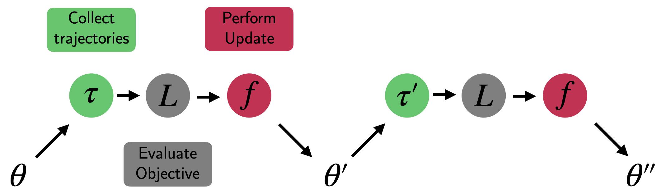
Fig. 1: Traditional first-order parameter update in RL: Collect, Evaluate, Update.
Now let’s assume that our update function explicitly depends on a set of meta-parameters $\eta$ (e.g. the discount factor $\gamma$):
\[\begin{aligned} \theta' = \theta + f(\tau, \theta, \eta). \end{aligned}\]Importantly, the update function is assumed to be differentiable with respect to $\eta$. We can then ask the following questions: How does the performance after the update depend on the meta-parameters used to perform the update? How should we choose $\eta$ for the next update given the current state of our agent? In order to answer this question, we need a meta-objective to evaluate a candidate $\eta$? One way to do so is to perform online cross-validation by (Sutton, 1992) using another hold-out trajectory $\tau’$, collected from the post-update policy. For simplicity, we can assume that the meta-objective $\bar{L}$, with which we evaluate $\eta$ on $\tau’$, is the same as the inner loop objective $L$ (e.g. some REINFORCE variant). Hence, we want to estimate the meta-gradient:
\[\begin{aligned} \frac{\partial \bar{L}(\tau', \theta', \bar{\eta})}{\partial \eta} &= \frac{\partial \bar{L}(\tau', \theta', \bar{\eta})}{\partial \theta'} \frac{d \theta'}{d \eta}. \end{aligned}\]
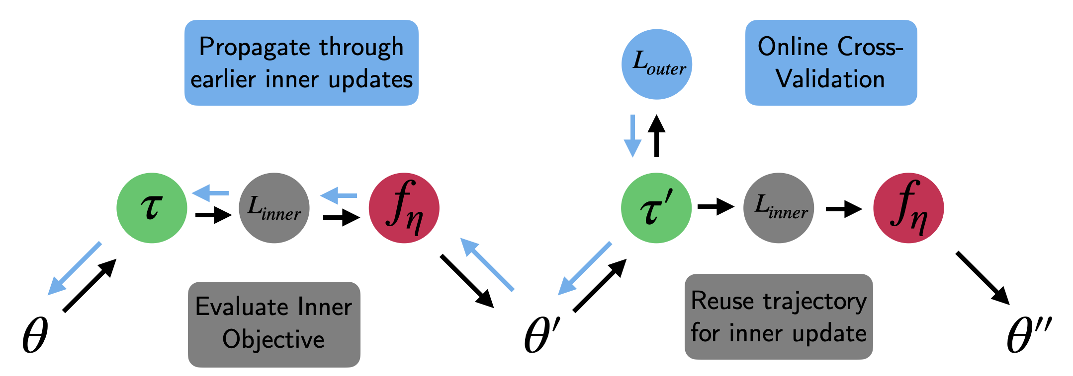
Fig. 2: Meta-Policy Gradient update based on online cross-validation.
Using the chain rule, we can re-write the derivative of the updated parameters $\theta’$ with respect to $\eta$:
\[\begin{aligned} \underbrace{\frac{d \theta'}{d \eta}}_{z'} &= \frac{d [\theta + f(\tau, \theta, \eta)]}{d \eta} = \frac{d \theta}{d \eta} + \frac{d f}{d \eta} + \frac{\partial f}{\partial \theta} \frac{d \theta}{d \eta} = \underbrace{(I + \frac{\partial f}{\partial \theta})}_{A} \underbrace{\frac{d \theta}{d\eta}}_{z} + \frac{\partial f}{\partial \eta}. \end{aligned}\]The dependence of the updated parameters on $\eta$ boils down to a dynamical system:
\[\begin{aligned} z' &= A z + \frac{\partial f}{\partial \eta}. \end{aligned}\]The parameters of this additive sequence and the respective Jacobians can be accumulated online as we unroll the network. This in turn provides us with all necessary ingredients to perform an outer loop gradient descent update to improve the hyperparameters $\eta$:
\[\begin{aligned} \Delta \eta = - \beta \frac{\partial{\bar{L}}}{\partial \theta'} \frac{d \theta'}{d \eta} = - \beta \frac{\partial{\bar{L}}}{\partial \theta'} \left[(I + \frac{\partial f}{\partial \theta}) \frac{d \theta}{d\eta} + \frac{\partial f}{\partial \eta}\right]. \end{aligned}\]Note that we have only considered the effect of the meta-parameters on the performance after a single update. Considering multiple steps is conceptually straight forward, but the math requires us to propagate gradients à la backpropagation through time. We can use a fixed set of $K$ steps and automatic differentiation toolboxes to do the gradient bookkeeping. The full meta-policy gradient procedure then boils down to repeating 3 essential steps (see figure 2):
- Update $\theta$ based on $\tau$ using the update function $f$ and $L$. Accumulate the resulting gradients into a trace $\{ z, z’, \dots \}$.
- Afterwards, cross-validate the performance of the updated agent on a new subsequent trajectory $\tau’$ using the meta-objective $\bar{L}$.
- Update the meta-parameters $\eta$ based on the meta-policy gradient $\frac{\partial{\bar{L}}}{\partial \eta}$ using SGD.
There are multiple resulting computational considerations: First, online cross-validation does not imply a decrease in sample efficiency. Instead of discarding $\tau‘$ after meta-evaluation, we can simply reuse it for step 1 of the next procedure iteration. Second, the derivative of the update $f$ with respect to the meta-parameters is expensive to compute. This is due to us having to to perform ‘unrolled’ optimization through a (multi-step) inner-loop optimization procedure. There is a set of heuristic solutions which result in a semi-/pseudo-meta policy gradient update:
- Using a cheap approximation to $\frac{df}{d\theta}$. This can be for example a diagonalized version.
- Using a decay factor, which exponential forgets about the importance of earlier updates.
- Fully truncating the sequence and only considering the influence of $\eta$ for a few steps.
And finally, the memory complexity of MPG increases with the ‘meta-trajectory length’ $K$. Choosing a small $K$ introduces a truncation bias, while larger $K$ may suffer from high variance. Furthermore, the trace of $z$ required to compute the meta-policy gradient may be tough to fit into memory (depending on the dimensionality of $\theta$ and $K$). Now that we have introduced the formal MPG framework, let’s see how we can exploit it.
MPGs for Online Deep RL Hyperparameter Tuning
The RL problem postulates an artificial agent, who maximizes its expected discounted cumulative reward. This reward is sampled from a stochastic and unkwown reward function. Hence, there is no simple and explicit differentiable objective as in the supervised learning case. Instead, we have to come up with a proxy objective such as the Mean-Squared Bellman Error or a Policy Gradient objective. These objectives come with their own hyperparameters, which often are non-trivial to tune and can require dynamic scheduling. MPG methods promise to discover adaptive objectives capable of providing the best possible proxy – at any given time of the learning procedure. Throughout the next section we will focus on how the MPG setup can improve the control problem using an actor-critic (AC) objective. We cover both the standard AC setup (Xu et al., 2018) as well as the IMPALA architecture (Zahavy et al., 2020).
Xu et al. (2018) - Meta-Gradient Reinforcement Learning
Paper |
Xu et al. (2018) applied the MPG framework to the return function $G_\eta(\tau_t)$ used throughout value-based RL and policy gradient baseline corrections. This includes the following formulations:
- The TD($0$) return: $G(\tau_t) = r_{t+1} + \gamma v_\theta(s_{t+1})$.
- The $n$-step Monte Carlo return: $G(\tau_t) = \sum_{i=1}^{n} \gamma^{i-1} r_{t+i} + \gamma^n v_\theta(s_{t+n})$.
- The TD($\lambda$) return: $G(\tau_t) = r_{t+1} + \gamma (1-\lambda) v_\theta(s_{t+1}) + \gamma \lambda G(\tau_{t+1})$,
where $v_\theta$ denotes a value estimator. The meta-parameters, $\eta = \{\gamma, \lambda\}$, control the bias-variance trade-off in RL. How much do we rely on Monte Carlo estimation and how much on a bootstrap estimate of future returns? $G$ defines the critic target and baseline corrects the REINFORCE term:
\[\begin{aligned} L_{ac}(\theta; \eta) &= L_{policy}(\theta) + g_v L_{value}(\theta) + g_e \mathbb{E}_\pi[\mathcal{H}(\pi_\theta(a|s))] \\ L_{value}(\theta) &= \mathbb{E}_\pi[(G_\eta(\tau) - v_\theta(s))^2]\\ L_{policy}(\theta) &= - \mathbb{E}_\pi[\log \pi_\theta(a | s) (G_\eta(\tau) - v_\theta(s))], \end{aligned}\]where $g_v$ and $g_e$ rescale the effective learning rate of the critic and entropy loss terms. The inner loop update $f$ for a fixed set of hyperparameters $\eta$ then boils down to:
\[\begin{aligned} \frac{\partial L(\tau, \theta, \eta)}{\partial \theta} =& - [G_\eta (\tau) - v_\theta(s)] \frac{\partial \log \pi_\theta}{\partial \theta} + g_v [G_\eta (\tau) - v_\theta(s)] \frac{\partial v_\theta}{\partial \theta} + g_e \frac{\partial \mathcal{H}}{\partial \theta}. \end{aligned}\]The next ingredient for our meta-policy gradient is the derivative of the update operation with respect to the meta-parameters $\eta$:
\[\begin{aligned} \frac{\partial f}{\partial \eta} = -\alpha \frac{\partial G_\eta(\tau)}{\partial \eta}[\frac{\partial \log \pi_\theta}{\partial \theta} + g_v \frac{\partial v_\theta}{\partial \theta}]. \end{aligned}\]Finally, the derivative of the online-validation loss wrt. the updated parameters is given by:
\[\begin{aligned}\frac{\partial \bar{L}}{\partial \theta'} = [G_ \eta(\tau') - v_\theta(s)] \frac{\partial \log \pi_{\theta'}}{\partial \theta'}. \end{aligned}\]We can now stitch all of these together, store our trace and update the meta-parameters $\gamma, \lambda$. Great! But there remains a fundamental challenge: Our inner-loop function approximators are shooting after a moving target. How can we learn values if the nature of the targets changes with each meta-parameter update? Here are a few solution ideas:
- Tune the learning rate scales (outer/inner loop ratios) or use trust region-constraint updates to ensure that the optimization procedure itself is sufficiently smooth in the meta-parameters.
- Xu et al. (2018) propose to not only learn the value function & policy for a single set of meta-parameters but for all $\eta$! Practically, this means that we provide an embedding of the meta-parameters as an input to the value/policy networks (as in UVFA; Schaul et al., 2015).
After the initial paper by Xu et al. (2018), this approach was extended to many more hyperparameters. Here is a list of references, which applies MPGs to a vast set of fundamental RL design choices:
| Paper | Tuned Parameters | Outer-Objective | Inner-Objective | Tasks |
|---|---|---|---|---|
| Xu et al. (2018) | Discount $\gamma$ & Bootstrap $\lambda$ | MSBE/Actor-Critic | REINFORCE | MRP, ATARI |
| Zheng et al. (2018) | Intrinsic Rewards | REINFORCE + IS | REINFORCE + Intrinsic | ATARI, MuJoCo |
| Veeriah et al. (2019) | Auxiliary Tasks | REINFORCE | REINFORCE + Answer Loss | ATARI |
| Wang et al. (2019) | Return Function | PPO + IS | REINFORCE | Gird, ATARI |
| Zhou et al. (2020) | Auxiliary Policy Updates | Tanh Diff. | DDPG | MuJoCo |
| Zahavy et al. (2020) | V-Trace, Coefficients, Aux. Tasks | Actor-Critic | Actor-Critic + Regularizer | ATARI |
Table 1: An Overview of MPG Methods for Hyperparameter Tuning.
Zahavy et al. (2020) - A Self-Tuning Actor-Critic Algorithm
Paper |
While these projects mainly focus on tuning small sets of hyperparameters, ultimately we would like to automatically tune the entire RL pipeline. Zahavy et al. (2020) make a big step into this direction by optimizing almost all hyperparameters of the IMPALA (Espeholt et al., 2018) architecture. But that’s not all: They also adapt the network architecture and objective to maximally utilize the power of MPGs. But let’s first take a step back: IMPALA is a large-scale off-policy actor-critic algorithm, which allows for high data throughput using the distributed actor-learner framework. Many workers asynchronously collect trajectories, which are then sent to a centralized learner. This learner processes the experience and performs gradient updates. There is one caveat: The trajectories are most likely not collected using the most recent policy. Therefore, the algorithm is not entirely on-policy and gradients (estimated from outdated policy rollouts) will become ‘stale’. IMPALA corrects for this covariate shift by using a procedure called v-trace. V-trace combats the off-policy nature of transitions with a modified importance sampling (IS) ratio, which explicitly controls the variance of the gradient estimators and contraction speed:
\[\begin{aligned} L_{policy}(\theta) &= - \sum_{s \in \tau} \rho_s \log \pi_\theta(a|s) [r + \gamma v_{v-trace}(s_{t+1}) - v_\theta(s)], \\ v_{v-trace}(s) &= v_\theta(s) + \sum_{j=0}^{s+n-1} \gamma^{j-s} (\prod_{i=s}^{j-1} c_i) \delta_j V, \\ \delta_j V &= \rho_j (r_j + \gamma v_\theta(s_{j+1}) - v_\theta(s_j)), \end{aligned}\]where $\rho_j$ controls the nature of the target value function by acting as a discount scaling. $c_i$, on the other hand, performs a form of trace cutting (à la Retrace, Munos et al., 2016). The clipping threshold $\bar{c}$ constrains the variance of the product of importance weights:
\[\begin{aligned} \rho_j &= \min \left(\bar{\rho}, \frac{\pi(a_j |s_j)}{\mu(a_j | s_j)}\right) \text{ and } c_i = \lambda \min \left(\bar{c}, \frac{\pi(a_j |s_j)}{\mu(a_j | s_j)} \right). \end{aligned}\]The IS ratio can be rewritten as $IS_t = \frac{\pi(a_j \mid s_j)}{\mu(a_j \mid s_j)}$. So where do MPGs come into play? The STAC algorithm (Zahavy et al., 2020) then aims to learn the degree of correction by utilizing a convex-combination version of the V-trace parameters:
\[\begin{aligned} \rho_t &= \alpha_\rho \min \left(\bar{\rho}, IS_t \right) + (1-\alpha_\rho) IS_t \\ c_t &= \lambda \left[\alpha_c \min(\bar{c}, IS_t) + (1-\alpha_c) IS_t \right]. \end{aligned}\]The meta-objective can then be differentiated with respect to $\alpha_\rho$, $\alpha_c$ and can smoothly interpolate between the fixed point of our approximate Bellman iteration for the target policy $\pi$ and the behaviour policy $\mu$. A low $\alpha_c$ puts more weight on IS, which in turn implies more contraction but also high variance. A large0 $\alpha_c$, on the other hand, emphasizes v-trace, which leads to less contraction but also lower variance. To stabilize the impact of the outer loop non-stationarity, Zahavy et al. (2020) modify the meta-objective and add a KL regularizer similar to TRPO:
\[\begin{aligned} \bar{L}(\tau', \theta', \eta) =& g_{p}^{outer} L_{policy}(\theta') + g_{v}^{outer} L_{value}(\theta') \\ & + g_{e}^{outer} L_{entropy}(\theta') + g_{KL}^{outer} KL(\pi_{\theta'} || \pi_\theta). \end{aligned}\]In order to assure the proper scaling between the inner and outer loss magnitude the authors propose to sigmoid-squash and scale the loss coefficients: $g_v = \sigma(g_v) \times g_v^{outer}$.
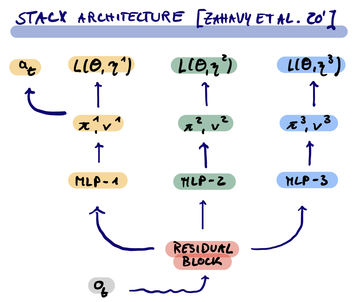 The second innovation of Zahavy et al. (2020) is to add a set of auxiliary output heads on top of the shared torso corresponding different policy and critic parameterization with their own meta-parameters. The meta-controller can then control the gradient flow into the torso for potentially different timescales. Only the first of the heads is used to generate the training trajectories, while the others act as implicit regularizers. The paper shows that on ATARI the MPG improvements increase, the more parameters we optimize with the MPG setup (panel B in figure 3).
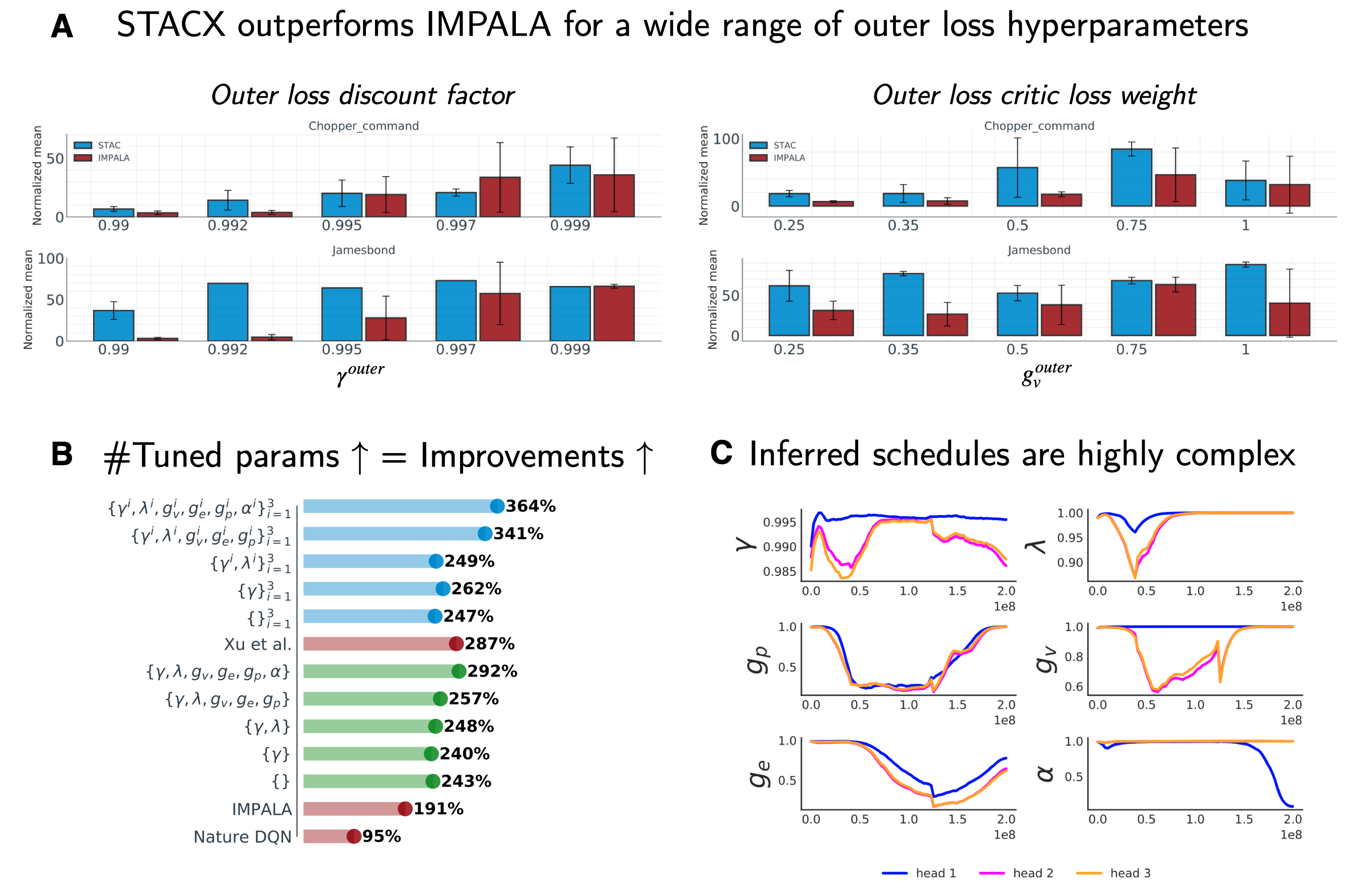
Fig. 3: STACX ATARI key results. Source: Adapted from Zahavy et al. (2020)
Empirically a high discount and value loss coefficient in the outer loop appear to perform better (panel A in figure 3). Finally, when examining the online optimized meta-parameter schedules on the James Bond ATARI game, we can see significant variation across the three heads and strong non-linear dynamics over the course of training (panel C in figure 3).
MPGs for Offline Discovery of Objective Functions
The RL problem is inherently misspecified. The agent is tasked with maximizing an expected sum of discounted rewards, without having access to the underlying reward function. In order to overcome this fundamental problem we define surrogate objectives. But it is safe to assume that for us humans the objective function changes over the course of our lives. Potentially making learning easier. Might it potentially even be possible to completely discard the ingenious legacy of Richard Bellman and to learn what to predict in order to best solve the RL problem? The ideas introduced in the following sections extend MPGs to not only optimize specific hyperparameters but to meta-optimize an entire parametrized surrogate objective function, which serves the purpose of providing the best learning curriculum to the RL agent. The first set of methods are offline and meta-learned across a large number of training inner-loops and different MDPs. Meta-learning a parametrized loss function $L_\phi$, has the advantage of potentially being more robust when varying the task distribution. The implicit characterization of the optimization problem allows for generalization beyond the meta-training distribution and tackles the core motivating problem: To disentangle learned learning algorithm from the learning agent.
Houthooft et al. (2018) - Evolved Policy Gradients (EPG)
Paper | Code
Computing higher-order gradients is expensive and truncating the unrolled optimization has the unwanted effect of introducing bias in the gradient estimates. In order to overcome this technical difficulty, Houthooft et al. (2018) propose to use evolutionary strategies for gradient estimation using a population of meta-loss parametrizations. The gradient of a (potentially non-differentiable) function $L$ is approximated using a population-based Monte Carlo estimator, e.g. via antithetic sampling:
\[\begin{aligned} \tilde{\nabla}_\phi \propto \frac{\beta}{2 \sigma^2 P} \sum_{i=1}^P \epsilon_i(L(\phi + \epsilon_i) - L(\phi - \epsilon_i)), \end{aligned}\]where $\epsilon_i \sim \mathcal{N}(0, \sigma^2 I)$. $P$ denotes the evaluated population size, $\sigma$ controls the perturbation variance and $\beta$ effectively rescales the learning rate. The individual function/network/agent evaluations can be collected in parallel. Houthooft et al. (2018) introduce a parametrization of the meta-loss, which uses temporal convolutions of the agents’ previous experiences. It takes into account the most recent history (see figure 4). The extended memory can help incentivize structured exploration in problems with long time horizons.
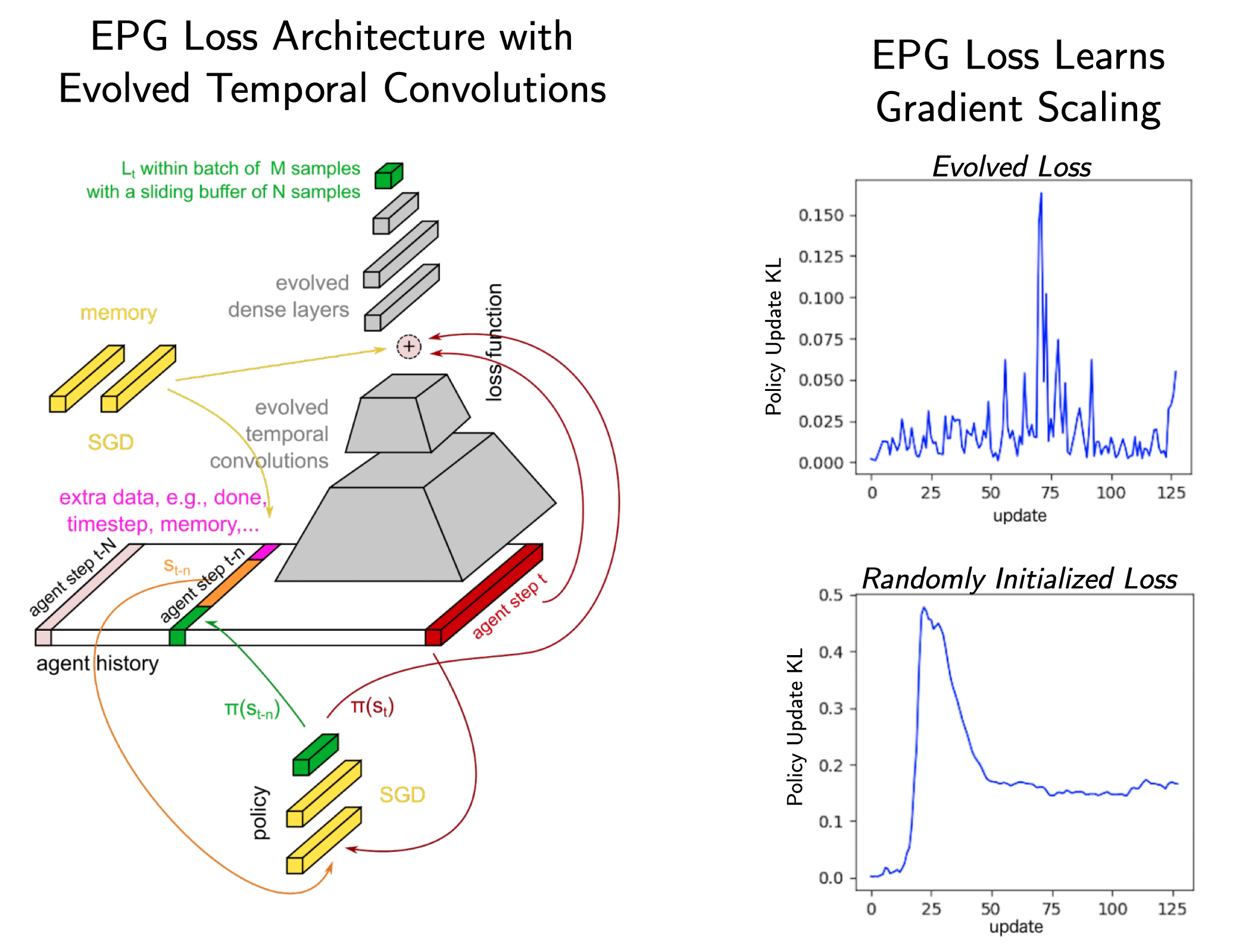
Fig. 4: EPG architecture. Source: Adapted from Houthooft et al. (2018)
Furthermore, the additional input may allow the loss to perform environment/task identification and to tail its target to a specific application. Furthermore, the meta-loss is fed a vector of ones, which can act as an explicit memory unit. During the inner loop optimization the agents uses the meta-loss to optimize their policy network parameters using standard SGD. The total loss of the inner loop is given by a convex combination of the parametrized loss and a standard PPO loss. A set of MuJoCo experiments reveal that EPG outperforms a plain PPO objective and that the resulting gradients are related but different (correlation of around 0.5). Interestingly, the authors find that the EPG loss has learned an adaptive gradient rescaling, which is reminiscent of policy update smoothness regularization ideas explicitly enforced in TRPO and PPO (see figure 4). One has to note that this comes at the substantial costs of an evolutionary outer-loop of meta-loss optimization. Finally, the authors show that one can combine the method with learned policy initializations such as MAML and that the loss does generalize to longer training horizons, different architectures as well as new tasks.
The general idea of an offline learned loss was afterwards extended by Chebotar et al. (2019), who use gradient-based meta-optimization and explicitly condition the meta-loss on additional task and context information. Interestingly, the authors show that the pre-conditioning can help shape the loss landscape for enhanced smoothness in the inner loop optimization.
Kirsch et al. (2020) - Improving Generalization in Meta Reinforcement Learning using Learned Objectives
Paper | Code
While the previous work mainly considered on-policy RL agents, Kirsch et al. (2020) extend meta-policy gradients to the off-policy setting, which allows to leverage replay buffers. As in ‘shallow’ non-meta RL this can lead to sample efficiency, since transitions are re-used multiple times to construct gradients. Conceptually, the proposed MetaGenRL framework builds on the off-policy continuous control algorithm DDPG (Lillicrap et al., 2015) and its extension TD3 (Fujimoto et al., 2018):
‘Our key insight is that a differentiable critic $Q_\theta: S \times A \to \mathbb{R}$ can be used to measure the effect of locally changing the objective function parameters $\alpha$ based on the quality of the corresponding policy gradients.’ - Kirsch et al. (2020, p.3)
So what does this mean on an algorithmic level? Standard DDPG alternates between minimizing a Mean-Squared Bellman Error of the critic $Q_\theta(s_t,a_t)$ and the improvement of the policy using the deterministic gradient of the value function wrt. the policy parameters ($\nabla_\phi \sum_{s_t} Q_\theta(s_t, \pi_\phi (s_t)$). In MetaGenRL an additional intermediate layer of transformation is added:
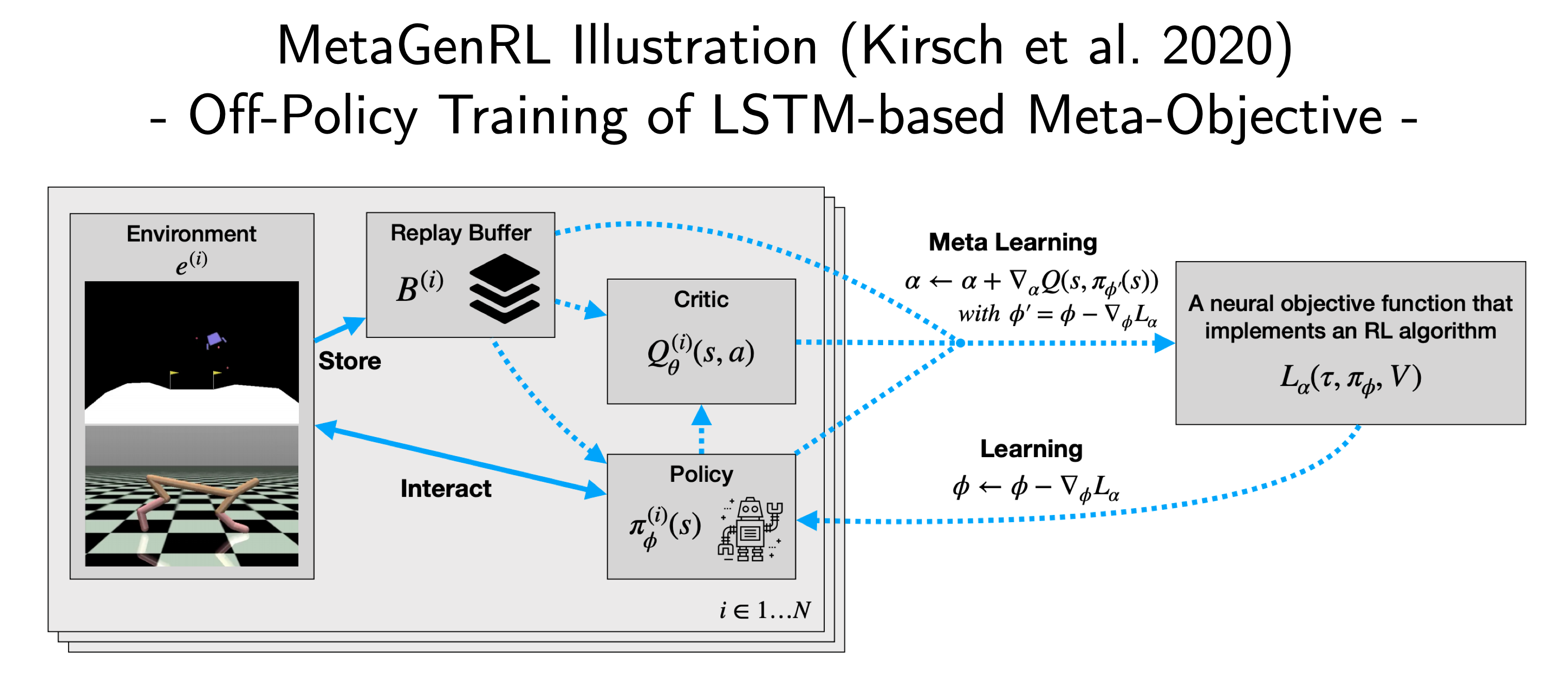
Fig. 5: MetaGenRL illustration. Source: Adapted from Kirsch et al. (2020)
The critic is now tasked to refine the objective function $L_\alpha$, which then in turn is used to construct policy gradients: $\nabla_\alpha Q_\theta(s_t, \pi_{\phi’}(s_t))$ with the policy update being prescribed by $L_\alpha$: $\phi’ = \phi - \nabla_\phi L_\alpha(\tau, x(\phi), V, t)$. Here, $x$ denotes additional auxiliary variables, which are a function of the policy. In practice, $L$ is parametrized by a small LSTM, which processes the trajectory data in reverse order. This allows the learned objective to evaluate a specific transition based on future experiences within an episode and to emulate a form of pseudo-bootstrapping. The authors benchmark on MuJoCo and against traditional meta-learning such as RL$^2$ and EPG. They find that MetaGenRL is not only more sample efficient and also allows for generalization to completely novel environments. Futhermore, they perform a set of ablation studies that show that the meta-objective performs well even without the timestamp input, but requires a value estimate input to induce learning progress.
Oh et al. (2020) - Discovering Reinforcement Learning Algorithms
Paper
Learned Policy Gradients (LPG, Oh et al., 2020) extend upon MetaGenRL in several aspects. Instead of relying on the notion of a critic, they overcome hand-crafted semantics by learning their own characterization of what might be important to predict on a set of representative Markov Decision Processes. They do not enforce any meaning on the agent’s vector-valued predictions. Instead the meta-learner decides what has to be predicted and thereby discovers its own update rules.
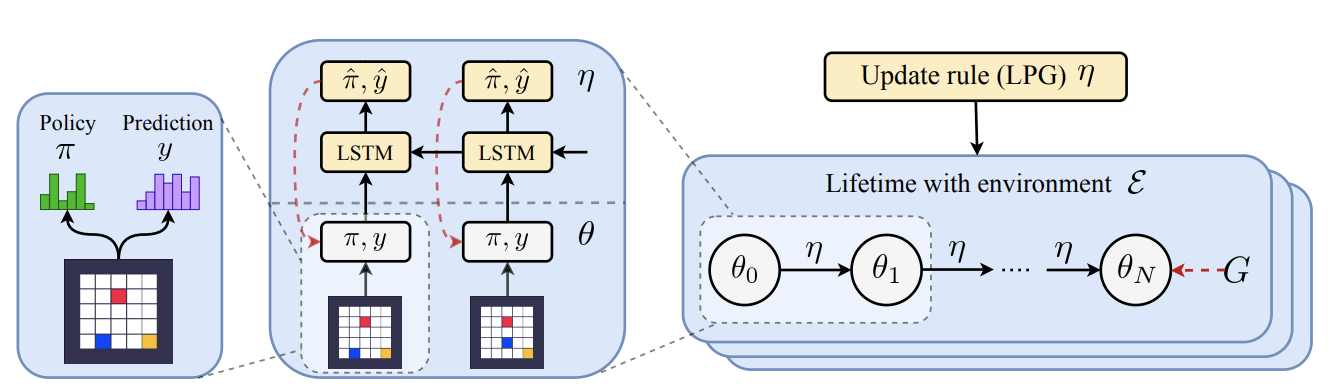
Fig. 6: Learned Policy Gradients schematic. Source: Oh et al. (2020)
The LPG framework proposes to use a recurrent neural network to emit inner loop optimization targets, $\hat{y}, \hat{\pi}$ (see figure 6). $\hat{\pi}$ denotes a policy-adjustment target, while $\hat{y}$ represents the output of a categorical distribution related to a specific state. Again, the RNN processes an episode in reverse order and is trained by performing gradient descent on a sequence of inner-loop gradient descent updates resulting from the previous objective parameterization. But unlike MetaGenRL it does not rely upon the notion of a value function for bootstrapping. $\hat{y}$ is free to learn its own semantics. The LPG targets can then be used to construct an inner loop update based on a combination of cross-entropy and KL divergence terms:
\[\begin{aligned} \Delta \theta \propto \mathbb{E}_{\pi_\theta}[\nabla_\theta \log \pi_\theta (a|s) \hat{\pi} - \alpha_y \nabla_\theta D_{KL}(y_\theta || \hat{y})]. \end{aligned}\]The KL loss term in the inner loop is reminiscent of ideas in Distributional RL such as C51 (Bellemare et al., 2017) and allows for a more detailed learning signal/belief estimate than the expected value. The outer loop loss is similar to the previously introduced objectives but also includes an additional set of regularizers, which aim to ensure stability throughout the optimization procedure wrt. to $\eta$, $\mid \mid \hat{\pi}\mid \mid_2^2$ and $\mid \mid \hat{y}\mid \mid_2^2$. In figure 7 panel A we can see how the different dimensions can encode different value-related estimates similar to classic value function bootstrapping.
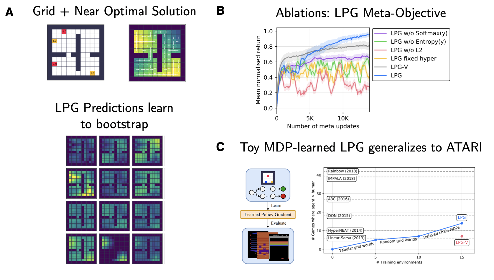
Fig. 7: Learned Policy Gradients key results. Source: Adapted from Oh et al. (2020)
Something that has left quite the impression on me, is the result depicted in figure 7 panel C: The authors show that it is possible to learn a target-providing RNN on a set of toy MDPs (gridworlds and delayed chain MDPs), which is capable of generalizing to ATARI almost as well as the substantially hand-tuned DQN objective with reward clipping and all the extra sauce. Since the underlying meta-training distribution of MDPs encode a set of fundamental RL problems (e.g. long-term credit assignment and the need for propagating state knowledge), the LPG is capable of substantial out-of-distribution generalization. Furthermore, adding more types of environments to the meta-train set improves the test performance of LPGs.
MPGs for Online Discovery of Objective Functions
The papers reviewed in the previous section are concerned with discovering objectives or parameter schedules offline. But can we also let MPGs discover potentially even better pillars to solve the RL problem online and during single optimization run?
Xu et al. (2020) - Meta-Gradient Reinforcement Learning with an Objective Discovered Online
Paper |
Xu et al. (2020) propose the FRODO algorithm, which has nothing to do with jewelry or Goblins, but stands for Flexible Reinforcement Objective Discovered Online. What makes FRODO special, is that the interplay between naive outer loss and involved inner loss is trained online within a single task and single agent’s lifetime. It does not require any task distribution or the capability to reset the environment. The target simply adapts as the agent experiences the world. Somewhat like real lifelong learning! As in the offline case, $\eta$ is no longer low dimensional, i.e. a single hyperparameter, but a neural net parametrizing the entire target return $G(\tau) = g_\eta(\tau)$.
\[\begin{aligned} \nabla_\theta L(\tau, \theta, \eta) \propto & (g_\eta(\tau) - v(s)) \nabla_\theta \log \pi(a|s) \\ & + c_1 (g_\eta (\tau) - v(s)) \nabla_\theta v(s)\\ & + c_2 \nabla_\theta \mathcal{H}(\pi(a|s)). \end{aligned}\]The inner loop target values do not have to encode the crucial Bellman consistency, i.e. that the current state value may be decomposed into reward and discounted next state value. Instead, this may (or may not) be discovered by the outer loop. You might imagine that training an entire network online might be even trickier in terms of non-stationary learning dynamics. And you are right. In order to overcome this (Xu et al., 2020) propose to add a prediction consistency regularizer on the meta-level:
\[\begin{aligned} \tilde{L}(\tau', \theta', \bar{\eta}) \leftarrow \bar{L}(\tau', \theta', \bar{\eta}) + c ||G_t^{\eta} - (R_{t+1} + \gamma G_{t+1}^\eta)||_2^2 . \end{aligned}\]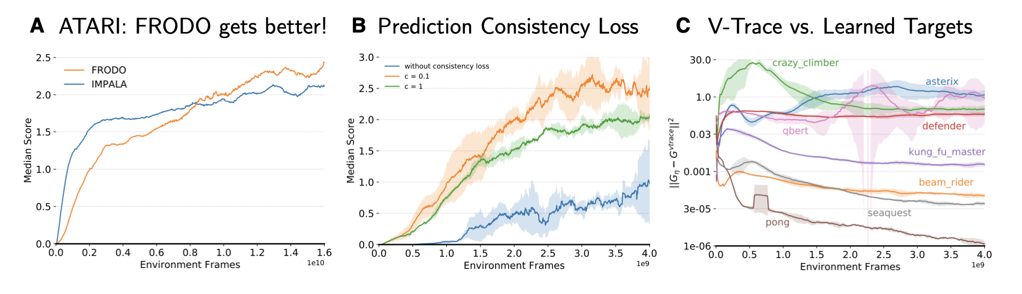
Fig. 8: FRODO key ATARI results. Source: Adapted from Xu et al. (2020)
The authors validate FRODO on the ATARI benchmark and panel A of figure 8 clearly indicates that the learning progress induced by FRODO improves throughout the learning process (exactly as in the cartoon sketch in the beginning of this post). Furthermore, an ablations study provides evidence for the importance of the consistency loss (panel B of figure 8). Finally, panel C shows how the learned targets vary across different ATARI games as well as the course of training. For some games FRODO learns to provide target returns close to v-trace (e.g. for simple games like Pong and Seaquest), while for other more challenging games learned return targets can differ quite significantly.
Open Research Questions
In this post we reviewed a set algorithms, which tune large parts of the RL pipeline using higher-order gradients. This enabled not only highly non-trivial training schedules but also to let the system decide what is important to learn at different stages of the process. How far can this hierarchical optimization paradigm be pushed? Here is a set of my personal open questions:
- How can we change architectures and the general RL setup to be ‘most tunable’? Adding additional output heads as in STACX is only one way, but there may be others. What is the set of environments which captures most of the dimensions of all relevant learning problems? Differently put – what should be the universal meta-training distribution?
- Schmidhuber’s vision of a self-referential learning system requires a notion of introspection, which goes beyond simple gradient-based learning. How can we push the current meta-learning setup closer to the theoretical optimal AIXI model?
- Rich Sutton wrote an opinionated blog ‘The Bitter Lesson’, which argues that most of the recent breakthroughs in machine learning were simply based on the drastic increase in computational resources. MPG fall under the same umbrella and increase the barrier to research. But how can we further reduce the compute requirements and increase sample efficiency?
Some Final Pointers & Acknowledgements
- David Silver’s workshop talk at ICML covering most of the DeepMind papers (07/20).
- Luke Metz’s great talk on learned optimizers and problems in unrolled optimization (08/20).
- Louis Kirsch’s talk at the NeurIPS 2020 meta-learning workshop (12/20).
- FAIR’s higher library, which supports higher-order gradient computation in PyTorch.
- DiCE trilogy on any-order score function estimation for RL: LoLA - Foerster et al. (2018a), DiCE - Foerster et al. (2018b), the blog post and Loaded DiCE - Farquhar et al. (2020).
You can find a pdf version of this post here. If you use it in your scientific work, please cite it as:
@article{lange2020_meta_policy_gradients,
  title   = "Meta Policy Gradients: A Survey",
  author  = "Lange, Robert Tjarko",
  journal = "https://roberttlange.github.io/year-archive/posts/2020/12/meta-policy-gradients/",
  year    = "2020",
  url     = "https://roberttlange.github.io/year-archive/posts/2020/12/meta-policy-gradients/"
}
References
- Andrychowicz, M., M. Denil, S. Gomez, M. W. Hoffman, D. Pfau, T. Schaul, B. Shillingford, and N. De Freitas. (2016): “Learning to Learn by Gradient Descent by Gradient Descent,” Advances in neural information processing systems, .
- Bellemare, M. G., W. Dabney, and R. Munos. (2017): “A distributional perspective on reinforcement learning,” arXiv preprint arXiv:1707.06887, .
- Chebotar, Y., A. Molchanov, S. Bechtle, L. Righetti, F. Meier, and G. Sukhatme. (2019): “Meta-learning via learned loss,” arXiv preprint arXiv:1906.05374, .
- Duan, Y., J. Schulman, X. Chen, P. L. Bartlett, I. Sutskever, and P. Abbeel. (2016): “Rl \^ 2: Fast reinforcement learning via slow reinforcement learning,” arXiv preprint arXiv:1611.02779, .
- Espeholt, L., H. Soyer, R. Munos, K. Simonyan, V. Mnih, T. Ward, Y. Doron, et al. (2018): “Impala: Scalable distributed deep-rl with importance weighted actor-learner architectures,” arXiv preprint arXiv:1802.01561, .
- Finn, C., P. Abbeel, and S. Levine. (2017): “Model-agnostic meta-learning for fast adaptation of deep networks,” arXiv preprint arXiv:1703.03400, .
- Flennerhag, S., A. A. Rusu, R. Pascanu, F. Visin, H. Yin, and R. Hadsell. (2019): “Meta-learning with warped gradient descent,” arXiv preprint arXiv:1909.00025, .
- Fujimoto, S., H. Van Hoof, and D. Meger. (2018): “Addressing function approximation error in actor-critic methods,” arXiv preprint arXiv:1802.09477, .
- Graves, A., G. Wayne, M. Reynolds, T. Harley, I. Danihelka, A. Grabska-Barwińska, S. G. Colmenarejo, et al. (2016): “Hybrid computing using a neural network with dynamic external memory,” Nature, 538, 471–76.
- Hochreiter, S., A. S. Younger, and P. R. Conwell. (2001): “Learning to Learn Using Gradient Descent,” International Conference on Artificial Neural Networks, Springer, 87–94.
- Houthooft, R., Y. Chen, P. Isola, B. Stadie, F. Wolski, O. A. I. J. Ho, and P. Abbeel. (2018): “Evolved Policy Gradients,” Advances in Neural Information Processing Systems, .
- Kirsch, L., S. van Steenkiste, and J. Schmidhuber. (2020): “Improving generalization in meta reinforcement learning using learned objectives,” arXiv preprint arXiv:1910.04098, .
- Lillicrap, T. P., J. J. Hunt, A. Pritzel, N. Heess, T. Erez, Y. Tassa, D. Silver, and D. Wierstra. (2015): “Continuous control with deep reinforcement learning,” arXiv preprint arXiv:1509.02971, .
- Metz, L., N. Maheswaranathan, J. Nixon, D. Freeman, and J. Sohl-Dickstein. (2019): “Understanding and Correcting Pathologies in the Training of Learned Optimizers,” International Conference on Machine Learning, .
- Metz, L., N. Maheswaranathan, C. D. Freeman, B. Poole, and J. Sohl-Dickstein. (2020): “Tasks, stability, architecture, and compute: Training more effective learned optimizers, and using them to train themselves,” arXiv preprint arXiv:2009.11243, .
- Munos, R., T. Stepleton, A. Harutyunyan, and M. Bellemare. (2016): “Safe and Efficient off-Policy Reinforcement Learning,” Advances in Neural Information Processing Systems, .
- Nichol, A., and J. Schulman. (2018): “Reptile: a scalable metalearning algorithm,” arXiv preprint arXiv:1803.02999, 2, 4.
- Oh, J., M. Hessel, W. M. Czarnecki, Z. Xu, H. van Hasselt, S. Singh, and D. Silver. (2020): “Discovering Reinforcement Learning Algorithms,” arXiv preprint arXiv:2007.08794, .
- Ritter, S., J. X. Wang, Z. Kurth-Nelson, S. M. Jayakumar, C. Blundell, R. Pascanu, and M. Botvinick. (2018): “Been there, done that: Meta-learning with episodic recall,” arXiv preprint arXiv:1805.09692, .
- Santoro, A., S. Bartunov, M. Botvinick, D. Wierstra, and T. Lillicrap. (2016): “Meta-Learning with Memory-Augmented Neural Networks,” International conference on machine learning, .
- Schaul, T., D. Horgan, K. Gregor, and D. Silver. (2015): “Universal Value Function Approximators,” International conference on machine learning, .
- Schmidhuber, J. (1987): “Evolutionary principles in self-referential learning,” On learning how to learn: The meta-meta-... hook.) Diploma thesis, Institut f. Informatik, Tech. Univ. Munich, 1.
- Sutton, R. S. (1992): “Adapting Bias by Gradient Descent: An Incremental Version of Delta-Bar-Delta,” AAAI, San Jose, CA, 171–76.
- Veeriah, V., M. Hessel, Z. Xu, J. Rajendran, R. L. Lewis, J. Oh, H. P. van Hasselt, D. Silver, and S. Singh. (2019): “Discovery of Useful Questions as Auxiliary Tasks,” Advances in Neural Information Processing Systems, .
- Wang, J. X., Z. Kurth-Nelson, D. Tirumala, H. Soyer, J. Z. Leibo, R. Munos, C. Blundell, D. Kumaran, and M. Botvinick. (2016): “Learning to reinforcement learn,” arXiv preprint arXiv:1611.05763, .
- Wang, Y., Q. Ye, and T.-Y. Liu. (2019): “Beyond Exponentially Discounted Sum: Automatic Learning of Return Function,” arXiv preprint arXiv:1905.11591, .
- Williams, R. J. (1992): “Simple statistical gradient-following algorithms for connectionist reinforcement learning,” Machine learning, 8, 229–56.
- Xu, Z., H. P. van Hasselt, and D. Silver. (2018): “Meta-Gradient Reinforcement Learning,” Advances in neural information processing systems, .
- Xu, Z., H. van Hasselt, M. Hessel, J. Oh, S. Singh, and D. Silver. (2020): “Meta-Gradient Reinforcement Learning with an Objective Discovered Online,” arXiv preprint arXiv:2007.08433, .
- Zahavy, T., Z. Xu, V. Veeriah, M. Hessel, J. Oh, H. van Hasselt, D. Silver, and S. Singh. (2020): “Self-Tuning Deep Reinforcement Learning,” arXiv preprint arXiv:2002.12928, .
- Zheng, Z., J. Oh, and S. Singh. (2018): “On Learning Intrinsic Rewards for Policy Gradient Methods,” Advances in Neural Information Processing Systems, .
- Zhou, W., Y. Li, Y. Yang, H. Wang, and T. M. Hospedales. (2020): “Online Meta-Critic Learning for Off-Policy Actor-Critic Methods,” arXiv preprint arXiv:2003.05334, .